HVDC

HVDC or high-voltage, direct current electric power transmission systems contrast with the more common alternating-current systems as a means for the bulk transmission of electrical power. The modern form of HVDC transmission uses technology developed extensively in the 1930s in Sweden at ASEA. Early commercial installations include one in the USSR in 1951 between Moscow and Kashira, and a 10-20 MW system in Gotland, Sweden in 1954^[1].

Advantages of high voltage transmission

Early electric power distribution schemes used direct-current generators located near the customer's loads. As electric power became more widespread, the distances between loads and generating plant increased. Since the flow of current through the distribution wires resulted in a voltage drop, it became difficult to regulate the voltage at the distribution circuit extremities.

Higher voltages reduce the transmission power loss or reduce the cost of conductors when transmitting a given quantity of power since a smaller current is required. Conductor cost is roughly proportional to the current carried, and conductor loss is roughly proportional to the square of the current, so higher transmission voltages improve the efficiency of transmission.

Low voltage is convenient for customer loads such as lamps and motors. The principal advantage of AC is that it allows the use of transformers to change the voltage at which power is used. No equivalent of the transformer exists for direct current, so the manipulation of DC voltages is considerably more complex. With the development of efficient AC machines, such as the induction motor, AC transmission and utilization became the norm (see War of Currents).

History of HVDC transmission

An early method of high-voltage DC transmission was developed by the Swiss engineer Rene Thury ^[2]. This system used series-connected motor-generator sets to increase voltage. Each set was insulated from ground and driven by insulated shafts from a prime mover. An early example of this system was installed in 1889 in Italy by the Society Acquedotto de Ferrari-Gallieri. This system transmitted 630 kW at 14 kV DC over a distance of 120 km^[3]. Other Thury systems operating at up to 100 kV dc operated up until the 1930s, but the rotating machinery required high maintenance and had high energy loss. Various other electromechanical devices were tested during the first half of the 20th century with little commercial success^[4].

The grid controlled mercury arc valve became available for power transmission during the period 1920 to 1940. In 1941 a 60 MW, +/- 200 kV, 115 km buried cable link was designed for the city of Berlin using mercury arc valves (Elbe-Project), but owing to the collapse of the German government in 1945 the project was never completed^[5]. The nominal justification for the project was that, during wartime, a buried cable would be less conspicuous as a bombing target. The equipment was moved to the Soviet Union and was put into service there ^[6].

Introduction of the fully-static mercury arc valve to commercial service in 1954 marked the beginning of the modern era of HVDC transmission. Mercury arc valves were common in systems designed up to 1975, but since then, HVDC systems use only solid-state devices.

Advantages of HVDC over AC Transmission

In a number of applications HVDC is often the preferred option.

• Undersea cables. (e.g. 250 km Baltic Cable between Sweden[[7]] and Germany[[8]].
• Endpoint-to-endpoint long-haul bulk power transmission without intermediate 'taps', for example, in remote areas.
• Increasing the capacity of an existing power grid in situations where additional wires are difficult or expensive to install.
• Allowing power transmission between unsynchronised AC distribution systems.
• Reducing the profile of wiring and pylons for a given power transmission capacity.
• Connection of remote generating plant to the distribution grid, for example Nelson River Bipole.
• Stabilising a predominantly AC power-grid,without increasing maximum prospective short circuit current.

Long undersea cables have a high capacitance. While this has minimal effect for DC transmission, the current required to charge and discharge the capacitance of the cable causes additional $I^{2}R$ power losses when the cable is carrying AC. In addition, AC power is lost to dielectric losses.

HVDC can carry more power per conductor, because for a given power rating the constant voltage in a DC line is lower than the peak voltage in an AC line. This voltage determines the insulation thickness and conductor spacing. This allows existing transmission line corridors to be used to carry more power into an area of high power consumption, which can lower costs.

Increased stability of power systems

Because HVDC allows power transmission between unsynchronised AC distribution systems, it can help increase system stability, by preventing cascading failures from propagating from one part to another of a wider power transmission grid, whilst still allowing power to be imported or exported in the event of smaller failures. This has caused many power system operators to contemplate wider use of HVDC technology for its stability benefits alone.

Possible health advantages of HVDC over AC transmission

A high-voltage DC transmission line would not produce the same sort of extremely low frequency (ELF) electromagnetic field as would an equivalent AC line. It is speculated by those who believe that ELF radiation is harmful that such a reduction in EM fields would be beneficial to health. The benefits would extend only to those near the transmission lines, as the electric and magnetic fields associated with high current AC transmission lines do not travel far beyond the actual lines themselves. These fields are, however, also associated with electrical equipment and household appliances. It should be noted that the current scientific consensus^[9] does not consider ELF sources and their associated fields to be particularly harmful, and that deployment of HVDC equipment would not completely eliminate electric fields, as there would still be DC electric field gradients between the conductors and ground.

Disadvantages

The required static invertors are expensive and cannot be overloaded very much. At smaller transmission distances the losses in the static inverters may be bigger than in an AC powerline, and the cost of the inverters may not be offset by reductions in line construction cost.

In contrast to AC systems, realizing multiterminal systems is complex, as is expanding existing schemes to multiterminal systems. Controlling power flow in a multiterminal DC system requires good communication between all the terminals.

AC network interconnections

AC transmission lines can only interconnect synchronized AC networks that oscillate at the same frequency and in phase. Many areas that wish to share power have unsynchronized networks. The power grids of the UK, Northern Europe and continental Europe all operate at 50 Hz but are not synchronized. Japan has 50 Hz and 60 Hz networks. Continental North America, while operating at 60Hz throughout, is divided into regions which are unsynchronised: East, West, Texas and Quebec. Brazil and Paraguay, which share the massive Itaipu hydroelectric plant, operate on 60Hz and 50Hz respectively. However, HVDC systems make it possible to interconnect unsynchronized AC networks, and also add the possibility of controlling AC voltage and reactive power flow.

A generator connected to a long AC transmission line may become unstable and fall out of synchronization with a distant AC power system. An HVDC transmission link may make it economically feasible to use remote generation sites. Wind farms located off-shore may use HVDC systems to collect power from multiple unsynchronized generators for transmission to the shore by an underwater cable.

In general, however, an HVDC power line will interconnect two AC regions of the power-distribution grid. Machinery to convert between AC and DC power adds a considerable cost in power transmission. The conversion from AC to DC is known as rectification, and from DC to AC as inversion. Above a certain break-even distance (about 50 km for under sea cables, and perhaps 600-800 km for overhead cables), the lower cost of the HVDC electrical conductors outweighs the cost of the electronics.

The conversion electronics also present an opportunity to effectively manage the power grid by means of controlling the magnitude and direction of power flow. An additional advantage of the existence of HVDC links, therefore, is potential increased stability in the transmission grid.

Rectifying and inverting

Rectifying and inverting components

Early static systems used mercury arc rectifiers, which were unreliable. Nevertheless some HVDC systems using mercury arc rectifiers are still in service in 2005. The thyristor valve was first used in HVDC systems in the 1960s. The thyristor is a solid-state semiconductor device similar to the diode, but with an extra control terminal that is used to switch the device on at a particular instant during the AC cycle. The insulated-gate bipolar transistor (IGBT) is now also used and offers simpler control and reduced valve cost.

Because the voltages in HVDC systems, up to 800 kV in some cases, exceed the breakdown voltages of the semiconductor devices, HVDC converters are built using large numbers of semiconductors in series.

The low-voltage control circuits used to switch the thyristors on and off need to be isolated from the high voltages present on the transmission lines. This is usually done optically. In a hybrid control system, the low-voltage control electronics sends light pulses along optical fibres to the high-side control electronics. Another system, called direct light triggering, dispenses with the high-side electronics, instead using light pulses from the control electronics to switch light-triggered thyristors (LTTs).

A complete switching element is commonly referred to as a 'valve', irrespective of its construction.

Rectifying and inverting systems

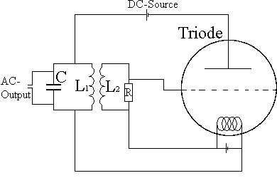
A simple DC to AC converter using 2 solenoids, a capacitor and a triode

Rectification and inversion use essentially the same machinery. Many substations are set up in such a way that they can act as both rectifiers and inverters. At the AC end a set of transformers, often three physically separate single-phase transformers, isolate the station from the AC supply, to provide a local earth, and to ensure the correct eventual DC voltage. The output of these transformers is then connected to a bridge rectifier formed by a number of valves. The basic configuration uses six valves, connecting each of the three phases to each of the DC rails. However, with a phase change only every sixty degrees, considerable harmonics remain on the DC rails.

An enhancement of this configuration uses 12 valves (often known as a twelve-pulse system). The AC is split into two separate three phase supplies before transformation. One of the sets of supplies is then configured to have a star (wye) secondary, the other a delta secondary, establishing a thirty degree phase difference between each of the sets of three phases. With twelve valves connecting each of the two sets of three phases to the two DC rails, there is a phase change every 30 degrees, and harmonics are considerably reduced.

In addition to the conversion transformers and valve-sets, various passive resistive and reactive components help filter harmonics out of the DC rails.

Configurations

Monopole and earth return

In a common configuration, called monopole, one of the terminals of the rectifier is connected to earth ground. The other terminal, at a potential high above, or below, ground, is connected to a transmission line. The earthed terminal may or may not be connected to the corresponding connection at the inverting station by means of a second conductor.

If no metallic conductor is installed, current flows in the earth between the earth electrodes at the two stations. The issues surrounding earth-return current include

• Electrochemical corrosion of long buried metal objects such as pipelines
• Underwater earth-return electrodes in seawater may produce chlorine or otherwise affect water chemistry.
• An unbalanced current path may result in a net magnetic field, which can affect magnetic navigational compasses for ships passing over an underwater cable.

These effects can be eliminated with installation of a metallic return conductor between the two ends of the monopolar transmission line. Since one terminal of the converters is connected to earth, the return conductor need not be insulated for the full transmission voltage which makes it less costly than the high-voltage conductor. Use of a metallic return conductor is decided based on economic, technical and environmental factors^[10].

Modern monopolar systems for pure overhead lines carry typically 1500 MW^[11]. If underground or seacables are used the typical value is 600 MW.

Bipolar

In bipolar transmission a pair of conductors is used, each at a high potential with respect to ground, in opposite polarity. Since these conductors must be insulated for the full voltage, transmission line cost is higher than a monopole with a return conductor. However, there are a number of advantages to bipolar transmission which can make it the attractive option.

• Under normal load, negligible earth-current flows, as in the case of monopolar transmission with a metallic earth-return; minimising earth return loss and environmental effects.
• When a fault develops in a line, with earth return electrodes installed at each end of the line, current can continue flow using the earth as a return path, operating in monopolar mode.
• Since for a given power rating bipolar lines carry only half the current of monopolar lines, the cost of the second conductor is reduced compared to a monopolar line of the same rating.
• In very adverse terrain, the second conductor may be carried on an independent set of transmission towers, so that some power may continue to be transmitted even if one line is damaged.

A bipolar system may also be installed with a metallic earth return conductor.

Bipolar systems may carry as much as 3000 MW at voltages of +/-533 kV. Under sea cable installations initially commissioned as a monopole may be upgraded with additional cables and operated as a bipole.

Back to back

A back-to-back station is a plant in which both static inverters are in the same area, usually even in the same building and the length of the direct current line is only a few meters. HVDC back-to-back stations are used for

• coupling of electricity mains of different frequency (as in Japan)
• coupling two networks of the same nominal frequency but no fixed phase relationship
• different frequency and phase number (for example, as a replacement for traction current converter plants)
• different modes of operation (as until 1995/96 in Etzenricht, Dürnrohr and Vienna).

In contrast to HVDC long-distance lines, the DC voltage in the intermediate circuit can be selected freely at HVDC back-to-back stations because of the short conductor length. The DC voltage is as low as possible, in order to build a small valve hall and to avoid parallel switching of valves. For this reason at HVDC back-to-back stations the strongest available static inverter valves are used.

Tripole - Current Modulating Control

A newly patented scheme (US Patent 6714427) is particularly applicable to conversion of existing AC transmission lines to HVDC. Two of the three circuit conductors are operated as a bipole. The third conductor is used as a parallel monopole, equipped with reversing valves (or parallel valves connected in reverse polarity). The parallel monopole periodically relieves current from one pole or the other, switching polarity over a span of several minutes. The bipole conductors would be loaded to either 1.37 or 0.37 of their thermal limit, with the parallel monopole always carrying +/- 1 times its thermal limit current. The combined RMS heating effect is as if each of the conductors was always carrying 1.0 of its rated current. This allows heavier currents to be carried by the bipole conductors, and full use of the installed third conductor for energy transmission. The higher current compared to AC operation may also help prevent ice build-up during winter storms. The system can be arranged to circulate high currents through the line conductors even if load demand is low.

Combined with the higher average power possible with a DC transmission line for the same line to ground voltage, a tripole conversion of an existing AC line could allow up to 80% more power to be transferred using the same transmission right-of-way, towers, and conductors. Some AC lines cannot be loaded to their thermal limit due to system stability, reliability, and reactive power concerns, which would not exist with an HVDC link.

The system operates without earth-return current. Since a single failure of a pole converter or a conductor results in only a small loss of capacity and no earth-return current, reliability of this scheme would be high. No time would be lost in switching if a conductor broke. The valves would inherently have an emergency overload rating in bipole mode. This would possibly allow great increase in power transmission with significant effect in congested transmission systems, where consequences of a single line failure limit the allowed loading of other parallel transmission lines. While capital costs are higher than for a bipole conversion operating at the same voltage class, the extra power capability reduces incremental cost per megawatt. Depending on transmission line physical configuration, replacement of insulators may be required to achieve the highest power rating, to insure proper line-to-line clearance distances.

As of 2005 no tri-pole conversions are in operation, although a transmission line in India has been converted to bipole HVDC.

See Presentation on Current-Modulated Control

United States Department of Energy comments received on an inquiry into power transmission bottlenecks

Corona discharge

Corona discharge is the creation of ions in a fluid (such as air) by the presence of a strong electric field. Electrons are torn from un-ionised air, and either the positive ions or else the electrons are attracted to the conductor, whilst the charged particles drift. This effect can cause considerable power loss, create audible and radio-frequency interference, generate toxic compounds such as oxides of nitrogen and ozone, and lead to arcing.

Both AC and DC transmission lines can generate coronas, in the former case in the form of oscillating particles, in the latter a constant wind. Due to the space charge formed around the conductors, an HVDC system may have about half the loss per unit length of a high voltage AC system carrying the same amount of power. With monopolar transmission the choice of polarity of the energised conductor leads to a degree of control over the corona discharge. In particular, the polarity of the ions emitted can be controlled, which may have an environmental impact on particulate condensation (particles of different polarities have a different mean-free path). Negative coronas generate considerably more ozone than positive coronas, and generate it further downwind of the power line, creating the potential for health effects. The use of a positive voltage will reduce the ozone impacts of monopole HVDC power lines.

Applications

Overview

The controllability of current-flow through HVDC rectifiers and inverters, their application in connecting unsynchronized networks, and their applications in efficient under sea cables mean that HVDC cables are often used at national boundaries for the exchange of power. Offshore windfarms also require undersea cables, and their turbines are unsynchronized. In very long-distance connections between just two points, for example around the remote communities of Siberia, Canada, and the Scandinavian North, the decreased line-costs of HVDC also makes it the usual choice. Other applications have been noted throughout this article.

The development of insulated gate bipolar transistors and gate turn-off thyristors has made smaller HVDC systems economical. These may be installed in existing AC grids for their role in stabilizing power flow without the additional short-circuit current that would be produced by an additional AC transmission line. One manufacturer calls this concept "HVDC Light", and has extended the use of HVDC down to blocks as small at a few tens of megawatts and lines as short as a few score kilometres of overhead line.

System configurations

A HVDC link in which the two AC-to-DC converters are housed in the same building, the HVDC transmission existing only within the building itself, is called a back-to-back HVDC link. This is the common configuration for interconnecting two unsynchronised grids or for changing frequency or for stabilizing an AC network.

HVDC back-to-back stations can also be designed to deliver single phase AC. This is required for Traction current converter plants.

The most common configuration of an HVDC link is a station-to-station link, where two inverter/rectifier stations are connected by means of a dedicated HVDC link. This is also a configuration commonly used in connecting unsynchronised grids, in long-haul power transmission, and in undersea cables.

Multi-terminal HVDC links, connecting more than two points, are rare. The configuration of multiple terminals can be series, parallel, or hybrid (a mixture of series and parallel). Parallel configuration tends to be used for large capacity stations, and series for lower capacity stations. An example is the 2000 MW Quebec - New England Transmission system opened in 1992, which is currently the largest multi-terminal HVDC system in the world^[12].

Realized HVDC systems

Systems that use (or used) mercury arc rectifiers

Name	Converter Station 1	Converter Station 2	Length of Cable	Length of overhead line	voltage	transmission power	inaugauration	remarks
Elbe-Project	Dessau, Germany	Berlin-Marienfelde, Germany	100 km	-	+-200kV	60 MW	1945	never placed in service, dismantled
Moscow-Kashira	Moscow, Russia	Kashira, Russia	100 km	-	200kV	30 MW	1951	built of parts of HVDC Elbe-Project, shut down
Gotland 1	Vaestervik, Sweden	Yigne, Sweden	98 km	-	200kV	20 MW	1954	shut down in February 1986
HVDC Cross-Channel	Echingen, France	Lydd, UK	64 km	-	+-100kV	160 MW	1961	shut down in 1984
Konti-Skan 1	Vester Hassing, Denmark	Lindome, Sweden	87 km	89 km	250kV	250 MW	1964
HVDC Volgograd-Donbass	Volzhskaya, Russia	Mikhailovskaya, Russia	-	475 km	+-400kV	750 MW	1964
HVDC Inter-Island	Benmore Dam, New Zealand	Haywards, New Zealand	40 km	570 km	+-250kV	600 MW	1965
HVDC back-to-back station Sakuma	Sakuma, Japan	Sakuma, Japan	-	-	+-125kV	300 MW	1965
SACOI 1	Suvereto, Italia	Lucciana, Corse; Codrongianos, Sardinia	304 km	118 km	200kV	200 MW	1965	multiterminal scheme
HVDC Vancouver Island 1	Delta, British Columbia	North Cowichan, British Columbia	42 km	33 km	260kV	312 MW	1968
Pacific Intertie	Celilo, Oregon	Sylmar, California	-	1362 km	+-500kV	3100 MW	1970	transmission voltage until 1984 +-400kV, maximum transmission power until 1982 1440 MW, from 1982 to 1984 1600 MW, from 1984 to 1989 2000 MW
Nelson River Bipole 1	Gillam, Canada	Rosser, Manitoba	-	895 km	+-450kV	1620 MW	1971	Used the largest mercury arc rectifiers ever built. Poles converted to thyristors in 1993, 2004.
HVDC Kingsnorth	Kingsnorth, UK	London-Beddington, UK; London-Willesden, UK	85 km	-	+-266kV	640 MW	1975	shut down

Systems that used thyristors from first power-on

Name	Converter Station 1	Converter Station 2	Length of Cable	Length of overhead line	voltage	transmission power	inaugauration	remarks
HVDC back-to-back station Eel River	New Brunswick, Canada	New Brunswick, Canada	-	-	80kV	320 MW	1972
Cross-Skagerak 1 + 2	Tjele, Denmark	Kristiansand, Norway	130 km	100 km	+-250kV	1000 MW	1977
HVDC Vancouver Island 2	Delta, British Columbia	North Cowichan, British Columbia	33 km	42 km	280kV	370 MW	1977
Square Butte	Center, North Dakota	Arrowhead, Minnesota	-	749 km	+-250kV	500 MW	1977
HVDC back-to-back station Shin Shinano	Shin Shinano, Japan	Shin Shinano, Japan	-	-	+-125kV	600 MW	1977
CU	Coal Creek, North Dakota	Dickinson, Minnesota	-	710 km	+-400kV	1000 MW	1979
HVDC Hokkaido-Honshu	Hakodate, Japan	Kamikita, Japan	44 km	149 km	250kV	300 MW	1979
Cabora Bassa	Songo, Mozambique	Apollo, South Africa	-	1420 km	+-533kV	1920 MW	1979
Inga-Shaba	Kolwezi, Zaire	Inga, Zaire	-	1700 km	+-500kV	560 MW	1964
HVDC back-to-back station Acaray	Acaray, Paraguay	Acaray, Paraguay	-	-	25,6 kV	50 MW	1981
HVDC back-to-back station Vyborg	Vyborg, Russia	Vyborg, Russia	-	-	+-85 kV	1065 MW	1982
HVDC back-to-back station Dürnrohr	Dürnrohr, Austria	Dürnrohr, Austria	-	-	145 kV	550 MW	1983	shut down in October 1996
HVDC Gotland 2	Västervik, Sweden	Yigne, Sweden	92.9 km	6.6 km	150 kV	130 MW	1983
HVDC back-to-back station Artesia, New Mexico	Artesia, New Mexico	Artesia, New Mexico	-	-	82 kV	200 MW	1983
HVDC back-to-back station Chateauguay	Châteauguay—Saint-Constant	Châteauguay—Saint-Constant	-	-	140 kV	1000 MW	1984
HVDC Itaipu 1	Foz do Iguaçu, Paraguay	São Rogue, Brasilia	-	785 km	+-600 kV	3150 MW	1984
HVDC Itaipu 2	Foz do Iguaçu, Paraguay	São Rogue, Brasilia	-	805 km	+-600 kV	3150 MW	1984
HVDC back-to-back station Oklaunion	Oklaunion	Oklaunion	-	-	82 kV	200 MW	1984
HVDC back-to-back station Blackwater, New Mexico	Blackwater, New Mexico	Blackwater, New Mexico	-	-	57 kV	200 MW	1984
HVDC back-to-back station Highgate, Vermont	Highgate, Vermont	Highgate, Vermont	-	-	56 kV	200 MW	1985
HVDC back-to-back station Madawaska	Madawaska	Madawaska	-	-	140 kV	350 MW	1985
HVDC back-to-back station Miles City	Miles City	Miles City	-	-	+-82 kV	200 MW	1985
Nelson River Bipole 2	Sundance, Canada	Rosser, Canada	-	937 km	+-500 kV	1800 MW	1985
HVDC Cross-Channel (new)	Les Mandarins, France	Sellindge, UK	72 km	-	+-270 kV	2000 MW	1986	2 bipolar systems
HVDC back-to-back station Broken Hill	Broken Hill	Broken Hill	-	-	+-8.33 kV	40 MW	1986
Intermountain	Intermountain, Utah	Adelanto, California	-	785 km	+-500 kV	1920 MW	1986
HVDC back-to-back station Uruguaiana	Uruguaiana, Brazil	Uruguaiana, Brazil	-	-	+-17.9 kV	53.9 MW	1986
HVDC Gotland 3	Västervik, Sweden	Yigne, Sweden	98 km	-	150 kV	130 MW	1987
HVDC back-to-back station Virginia Smith	Sidney, Nebraska	Sidney, Nebraska	-	-	55.5 kV	200 MW	1988
Konti-Skan 2	Vester Hassing, Denmark	Stenkullen, Sweden	87 km	60 km	285 kV	300 MW	1988
HVDC back-to-back station Mc Neill	Mc Neill, Canada	Mc Neill, Canada	-	-	42 kV	150 MW	1989
HVDC back-to-back station Vindhyachal	Vindhyachal, India	Vindhyachal, India	-	-	176 kV	500 MW	1989
HVDC Sileru-Barsoor	Sileru, India	Barsoor, India	-	196 km	+-200 kV	400 MW	1989
Fenno-Skan	Dannebo, Sweden	Rauma, Finland	200 km	33 km	400 kV	500 MW	1989
HVDC Gezhouba - Shanghai	Gezhouba, China	Nan Qiao, China	-	1046 km	+-500 kV	1200 MW	1989
Quebec - New England Transmission	Radisson, Quebec	Nicolet, Quebec; Des Cantons, Quebec; Comerford, New Hampshire; James Bay, Massachuses	-	1100 km	+-450 kV	2000 MW	1991	multiterminal scheme
HVDC Rihand-Delhi	Rihand, India	Dadri, India	-	814 km	+-500 kV	1500 MW	1992
SACOI 2	Suvereto, Italia	Lucciana, France; Codrongianos, Italy	118 km	304 km	200 kV	300 MW	1992	multiterminal scheme
HVDC Inter-Island 2	Benmore Dam, New Zealand	Haywards, New Zealand	40 km	570 km	350 kV	640 MW	1992
Cross-Skagerak 3	Tjele, Denmark	Kristiansand, Norway	130 km	100 km	350kV	500 MW	1993
Baltic-Cable	Lübeck-Herrenwyk, Germany	Kruseberg, Sweden	250 km	12 km	450 kV	600 MW	1993
HVDC back-to-back station Etzenricht	Etzenricht, Germany	Etzenricht, Germany	-	-	160 kV	600 MW	1993	shut down in October 1995
HVDC back-to-back station Vienna-Southeast	Vienna, Austria	Vienna, Austria	-	-	142 kV	600 MW	1993	shut down in October 1996
HVDC Haenam-Cheju	Haenam, South Korea	Jeju, South Korea	101 km	-	180 kV	300 MW	1996
Kontek	Bentwisch, Germany	Bjaeverskov, Denmark	170 km	-	400 kV	600 MW	1996
HVDC Hellsjön-Grängesberg	Hellsjoen, Sweden	Graengesberg, Sweden	-	10 km	180 kV	3 MW	1997	experimental HVDC
HVDC back-to-back station Welch-Monticello	Welch-Monticello, Texas	Welch-Monticello, Texas	-	-	162 kV	600 MW	1998
HVDC Leyte - Luzon	Orno, Leyton	Ormoc, Luzon	21 km	430 km	350 kV	440 MW	1998
HVDC Visby-Nas	Nas, Sweden	Visby, Sweden	70 km	-	80 kV	50 MW	1999
Swepol	Starnö, Sweden	Slupsk, Poland	245 km	-	450 kV	600 MW	2000
HVDC Italy-Greece	Galatina, Italy	Arachthos, Greece	200 km	110 km	400 kV	500 MW	2001
Kii Channel HVDC system	Anan, Japan	Kihoku, Japan	50 km	50 km	+-500 kV	1400 MW	2000
HVDC Moyle	Auchencrosh, UK	Ballycronan More, UK	63.5 km	-	250 kV	250 MW	2001
HVDC Thailand-Malaysia	Khlong Ngae, Thailand	Gurun, Malaysia	-	110 km	300 kV	300 MW	2002
HVDC back-to-back station Minami-Fukumitsu	Minami-Fukumitsu, Japan	Minami-Fukumitsu, Japan	-	-	125 kV	300 MW	1999
HVDC Three Gorges-Changzhou	Longquan, China	Zhengping, China	-	890 km	+-500 kV	3000 MW	2003
HVDC Three Gorges-Guangdong	Jingzhou, China	Huizhou, China	-	940 km	+-500 kV	3000 MW	2003
Basslink	Loy Yang, Australia	George Town, Australia	298.3 km	71.8 km	400 kV	600 MW	2005
NorNed	Feda, Norway	Eemshaven, Netherlands	580 km	-	+-450 kV	700 MW	2010
HVDC back-to-back station at Vishakapatinam	Vishakapatinam, India	Vishakapatinam, India	-	-

Systems that used IGBTs from first power-on

Name	Converter Station 1	Converter Station 2	Length of Cable	Length of overhead line	voltage	transmission power	inaugauration	remarks
HVDC Tjæreborg	Tjæreborg, Denmark	Tjæreborg, Denmark	4.3 km	-	+-9 kV	7,2 MW	2000	interconnection to wind power generating stations
Directlink	Mullumbimby, Australia	Bungalora, Australia	59 km	-	+-80 kV	180 MW	2000	land cable
Cross Sound Cable	New Haven, Connecticut	Shoreham, Long Island	40 km	-	+-150 kV	330 MW	2002
Murraylink	Berri, Australia	Red Cliffs, Australia	177 km	-	+-150 kV	220 MW	2002	land cable
HVDC Troll	Kollsnes, Norway	Offshore platform Troll A	70 km	-	+-60 kV	84 MW	2005	power supply for offshore gas compressor
Estlink	Espoo, Finland	Harku, Estonia	105 km	-	+-150kV	350 MW	2006

See also

• Static inverter plant
• Valve hall
• Electrode line
• Electrical pylon
• Uno Lamm

References

1. ^  Narain G. Hingorani in IEEE Spectrum magazine, 1996.
2. ^  Donald Beaty et al, "Standard Handbook for Electrical Engineers 11th Ed.", McGraw Hill, 1978
3. ^  http://www.myinsulators.com/acw/bookref/histsyscable/
4. ^  Shaping the Tools of Competitive Power http://www.tema.liu.se/tema-t/sirp/PDF/322_5.pdf
5. ^  http://www.rmst.co.il/HVDC_Proven_Technology.pdf
6. ^  http://www.ieee.org/organizations/history_center/Che2004/DITTMANN.pdf
7. ^  ABB HVDC website
8. ^  Scientific Facts on electromagnetic fields from Power Lines, Wiring & Appliances
9. ^  Basslink project
10. ^  Siemens AG "HVDC Basics" page.
11. ^  ABB HVDC Transmission Québec - New England website

• History of HVDC
• World Bank briefing document about HVDC systems